Machine Learning
Credit Risk with Wavelet Attributes
Executive Summary
The goal of this project is to determine whether using features with time series patterns, instead of using static features,
can better predict the likelihood of consumer default. The data available to us include customers’ attributes (size of3000),
demography information, trade line scores information, and bankruptcy records.
To construct time series attributes, we first decided to use 32 months as the time window to observe.
Then, we chose six time series feature from Equifax database that contains the trade line information of the customers,
and synthesized a new set of features using wavelet transformation. These wavelet attributes characterize the original time series
by measuring the similarity between the time series and a set of predefined patterns.
By using wavelet transformation, we transformed the data table into new wavelet transformed attributes.
After getting these two different attributes tables, we wanted to evaluate these two attributes by the same binary classification model —
CART(Classification and Regression Tree) on them. By comparing the predicting performance of using ADAs and wavelet attributes independently,
we found that the model using wavelet attributes provides a decent result, and it nearly matches the performance of using ADAs.
Wavelet Attributes
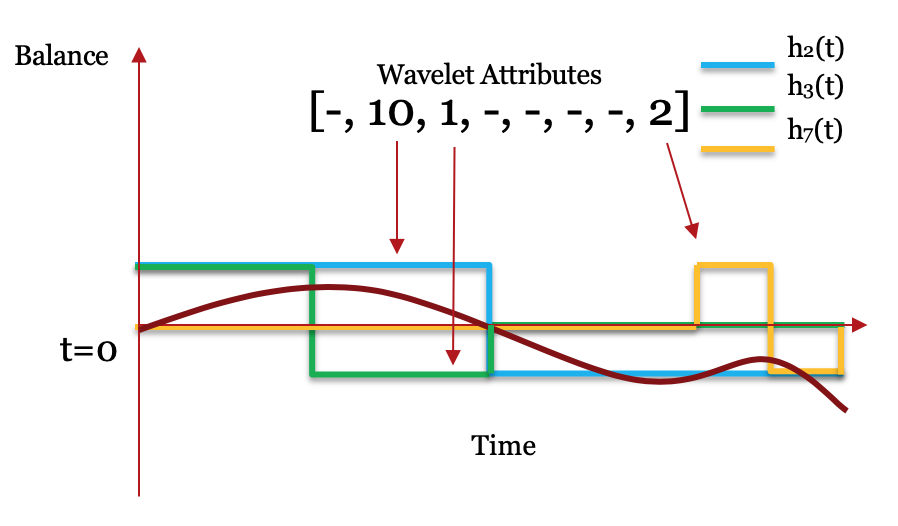
A wavelet is a function that has a wavelike graph. For any time series, we can calculate the inner product between the time series and a predefined wavelet function to measure the similarity between them.
For example, if we have the data of a bank account balance \(B(t)\) over a period of time \(t_i, i=0, 1, \cdots, n\), as shown in the figure below,
and we want to know whether the balance is higher in the first half or in the second, then we can just compare the summation of the first half of the observations and the summation of the second half.
This process directly corresponds to calculating the inner product between the balance time series and the wavelet function \(W(t)\) shown in the figure below. For this specific example,
the first half of the balance time series is all positive and the second half is all negative, which matches well with the wavelet function.
Thus, the result of the inner product \(\langle B(t), W(t) \rangle = \Sigma_{i=0}^n B(t_i)W(t_i)\) will be relatively high. Also, if the balance starts at a low level and increases significantly,
then the inner product should be a large negative number.
A natural extension of this idea is using the inner product to measure the similarity between a time series and a series of wavelet functions simultaneously.
Given a set of $k$ wavelet functions \(W_1(t), W_2(t), \cdots W_k(t)\), we can characterize the original time series by a vector of its similarity with the \(k\) wavelet functions.
For example, we can transform the balance time series \(B(t)\) into a vector $$(\langle B(t), W_1(t) \rangle, \langle B(t), W_2(t) \rangle, \cdots,\langle B(t), W_n(t) \rangle)$$
This process is called the wavelet transformation. Our hypothesis is that wavelet transformation can help better characterizing a time series and can synthesize new features with high predictive power.

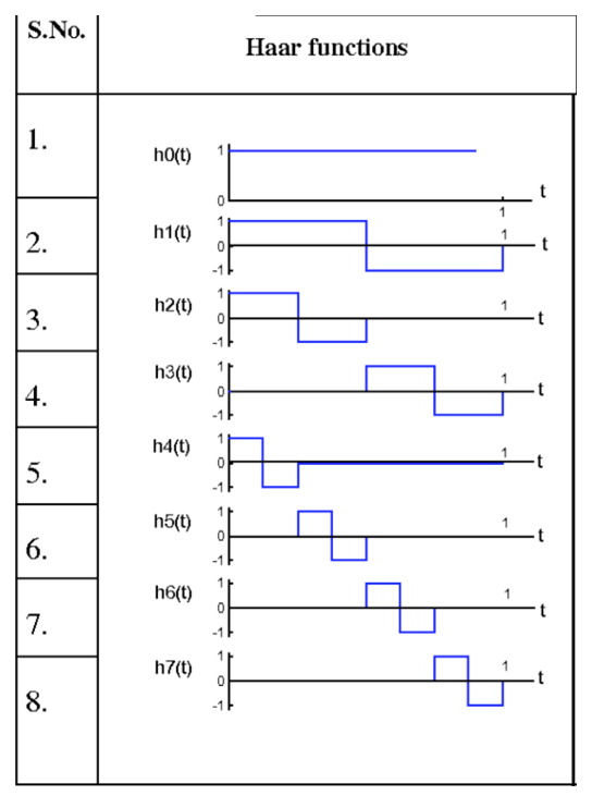
Haar Wavelet
There are many different kinds of wavelet series. For simplicity and interpretability, we chose the Haar wavelet proposed in 1909 by Alfréd Haar. The following figure on the right is a visualization of Haar wavelet of order 3. There are 3 different scaling levels and \(2^3 = 8\)wavelet functions in total. Except for the first wavelet function, which is a horizontal line, all wavelet functions are square waves with only one peak and one valley. Besides, all square waves share the same shape but have different scales and offset. For instance, wavelet function No. 2, 3, 5 have the same offset of 0, but they individually have a scaling level of 1, 2, and 3. Wavelet function No. 2 is a pattern on the entire domain of the time series, while wavelet function No. 3 is a pattern only in the first half of the domain, and wavelet function No. 5 is a pattern only in the first quarter of the domain. On the other hand, wavelet function No. 5, 6, 7, 8 has the same scale but different offset. Figure on the left below illustrates the partial result of Haar wavelet transformation on the balance time series.
Attribute overview
For this project, we only used two data tables, which are Trades and Attributes.
The Trades table contains trade line information for customers including account type, balance, payment behavior, and more.
The Attributes table has 571 \textbf{ADA}s (Advanced Decision Attributes) covering many attributes of applicants.
We will give a detailed explanation of the two tables in later sections.
In the Trades table, there are 5 features including Balance, Schedule Payment, Actual Payment, High Credit, and Credit Limit.
We crafted and additional feature, which is number of active accounts for a particular account type, to this table.
Then we applied MODWT to the 6 features to get the table that will be used in the modeling part.
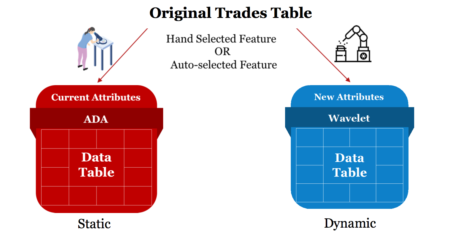
From the Attributes, we selected 141 ADAs by hand, which we believed to contain the same amount of information
as the trade line features that we used for wavelet transformation, out of the whole 571 ADA features from Attributes table.
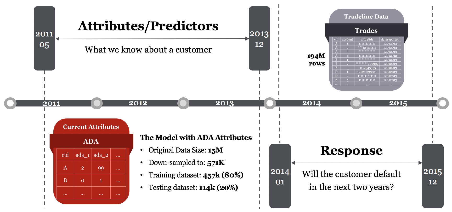
Figure below explains our two data tables. The red table is the 141 ADA features,
while the blue table is the MODWT-transformed features.
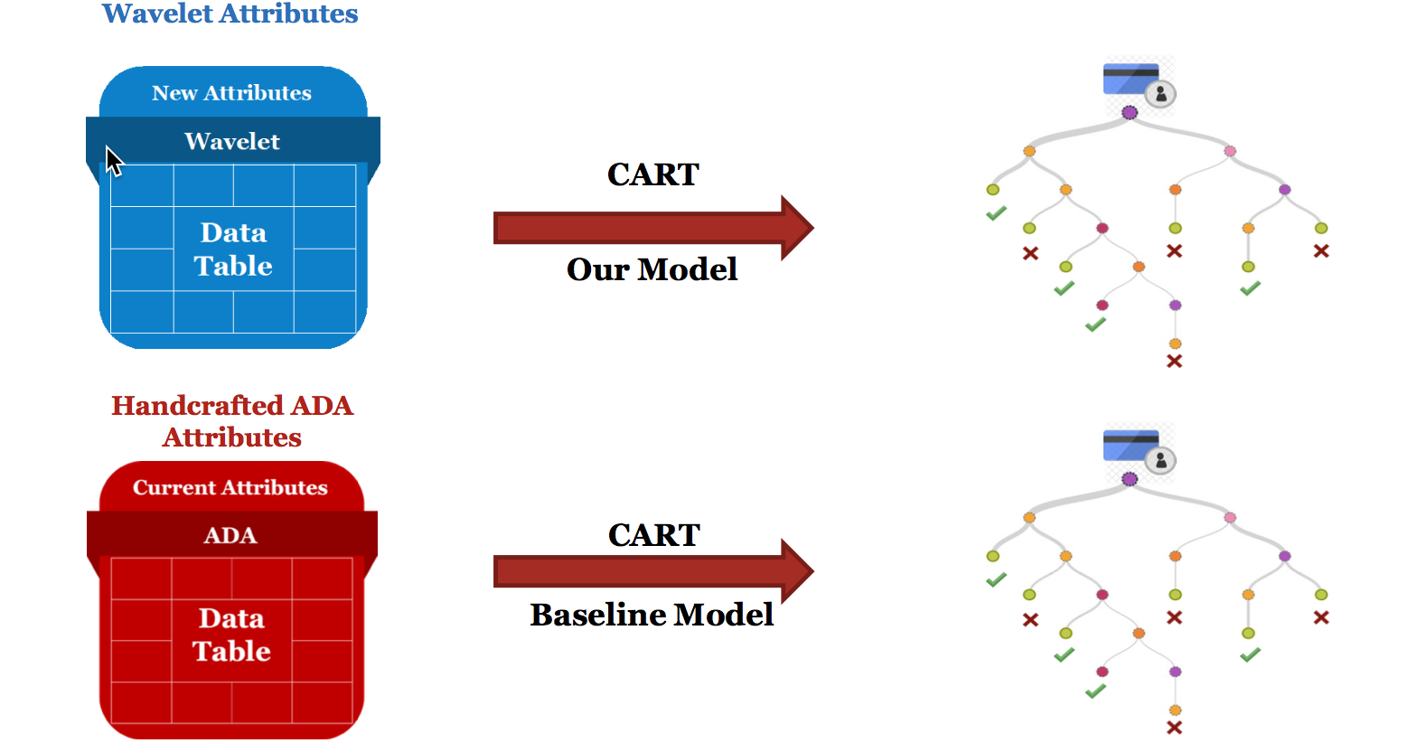
CART(Classification and Regression Tree)
is a tree-based model that can be used in both classification and regression.
We expect that CART can help us to build a model with high interpretability and robustness.
Figure below explained our two processes. To compare the predicting power of the two tables,
we applied CART to both tables.
Data Analysis and Exploration
For this project we only used two data tables, which are Trades and Attributes.
In the Attributes table, each line stands for a customer, and there are roughly $15$ million consumers.
The Trades table contains trade line information for customers including account type,
balance, payment behavior, and etc., and the data size is about 194 million.
As we could see in figure below, our raw data included attributes (the applicants' historical features)
and trades (the applicants' historical behaviors) from January 2011 to December 2015. To illustrate the data we used,
ADAs involves many attributes of every applicant in every month from January 2011 to December 2015, and
rades involves the default behavior vector (of length 48 which stands for 48 months) of every account of every applicant
in every month from January 2011 to December 2015, presented in number of 1-9, called grid48dr.
Figure below shows the the possible values in grid48 and their corresponding meanings.
A number above or equals to 4 in a particular month in grid48dr would be considered as applicant
default in that month.
Time Series Analysis
In this section, we explored more details on how we built the time series attribute table and use wavelet transformation transform the time series variables into static attributes by wavelet transformation. After we obtained the transformed data table, we then classified consumers' accounts by binary classification models.
Construction of Time Series Attribute Table
We chose 5 features from trades table, namely Balance, Schedule Payment, Actual Payment, High Credit and Credit Limit. A small number of attributes are easy to calculate in wavelet transformation. Moreover, we also created a manual feature, the number of active accounts for a particular account type. By looking at the date-open and date-closed time data, we could find the number of accounts open at any time point. Therefore, these 6 variables provide a basis for time series data table establishment and wavelet transformation.
We created a panel data set that is a multidimensional data set involving measurement over time. Each customer ID and a particular account type has 6 time series variables. For example, from the figure 1, cid 1 (a customer) has a Revolving (R) account type and there are 6 time series variables for that account from month 1 to month 32. The form that contain both variables and time is called panel data.
![]()
Maximal Overlap Discrete Wavelet Transformation
In section 2, we have introduced the Maximal Overlap Discrete Wavelet Transform (MODWT), which is an improvement of the Haar Wavelet transformation. We obtained a MODWT-transformed attributes table with 1920 columns. Then we split the column of the table and moved the offset structure from columns to rows and formed a panel table with 60 columns and 32 times more rows. To be more specific, the transformed attributes \(W\) would have \(6 \cdot 5\cdot 2\) columns, which contained 6 features, 5 levels of scaling for each feature, 2 types of transformation functions (scaling functions \(\Phi\) and wavelet functions \(W(t)\). The number of rows of the matrix is the number of the combination of consumers and account type in the cohort multiplies 32 time window length. Figure 2 illustrates the outcome of MODWT tranformed data table. In this MODWT attributes table, for each cid, type and time combination, there are 60 attributes. Each row represents how well the corresponding consumer's 6 credit behavior time series matched with a particular pattern corresponds to a wavelet functions. This table is used for further modeling.
![]()
Modeling
For MODWT transformed data, We also constructed a CART model to compare with the baseline model on 141 ADAs. By using exactly the same protocol for cross validation, we found the model with maximal depth 15 and minimal number of leaf is l has the best accuracy on testing set. The AUC for this model is 0.780 and the KS is 0.441.
Baseline CART Model
CART, a tree-based classification model using Gini impurity to split decision branches, can be used for baseline ADAs attributes and MODWT-transformed attributes. The gain in purity during each split indicates the importance of the feature. We expect that CART can help us to build a model with high interpretability and robustness.
CART is easy to interpret. The decision process of CART can be viewed as climbing a tree from the root to a leaf node. At each intersection, a question will be asked to determine which branch to go for the next step. Once a leaf node is arrived, the decision corresponding to that node will be the final result. Therefore, if an observation is predicted as true or false by the CART, then we can trace the path passed by that observation on the decision tree and conclude which traits in that observations leads to the final result. This feature of CART allows it to easier comply with current legal regulation on credit risk prediction. Because if a customer complains the result of credit card application being rejected by a automated process, the provider of the model can give specific feedback and explanation regarding why the customer is rejected and what should he or she do to restore a better credit history.
CART allows us to do the cross validation using different combination of hyper-parameter to find the most model. For each combination of hyper-parameter, we trained a CART model with the training set and estimate its accuracy on the validation set. After selecting the best combination of hyper-parameters, we trained a new CART model on the training and validation set and measured its performance on the test set.
We hand-selected 141 ADA features which we believed to contain the same amount of information as the trade line features that we used for wavelet transformation, out of total 571 ADA features, and used only features from May 2011 to December 2013 as the wavelet-transforming method requires only data of 32 months from May 2011 to December 2013. Then we put the 141 ADA features into CART model to build our baseline model to predict the default behavior of applicants in the next two years. The response in training and testing should be a true/false value indicating whether the applicant had defaulted for at least one time in the next two years (e.g., from January 2014 to December 2015). Since we were not given the label, we needed to look at last 24 digits (2 years) in the grid48 and label those customers who had any historical default record as default and others as non-default.
Since CART assumes balanced data set, we downsampled the negative (e.g., not default) class in training set so that the negative and positive classed in the training set were of the same size. After all the prerequisition is finished, we try to use CART to build the classification model.
After applying cross validation, we found the model with maximal depth 15 and minimal number of leaf is l outperform others. We tested the model performance on both ROC and KS. Usually, ROC is used to measure the overall prediction accuracy of a binary classification model. And KS is used to compare the accuracy between a model and random guessing. For both statistics, higher is better.
The test result of the CART model with cross validation is in the following table, with overall AUC 0.820 and KS 0.54. Here KS is defined as the maximum vertical distance between the ROC and the line \(y=x\). Also, ROC of CART model is presented in Figure

Final Conclusion
In this project, we tried to generate a set of new features from credit time series by wavelet transformation. we successfully converted time series attributes into shape-based descriptive attributes automatically using MODWT fo Haar wavelet transformation. We found that using this automatic attributes generation method could achieve similar result comparing to the handcrafted attributes (ADAs). This method not only does not presume any domain knowledge but also more cost-efficient than ADAs attributes.