NLP
In this report we first explore the data set, drop useless information in the data and explore the correlation between the features and the label. Then for classification we use Logistic regression and two tree based methods (Random Forest and XGBoost) to predict whether the customer spent money on the website. Cross validation are used for selecting hyper parameters for each model and we compare their performance by Mean Square Error.
For regression we try linear regression (including feature selection), tree based methods (bagging and boosting) and neural network solution. We hope to get a much smaller mean square error compared to the variance of the data.
Then we use the best models from both classification (XGboost) and regression (ridge regression) to build a combined model, and improve the result by using predicted data to train the regression model. The new hybrid model has a MSE of 1.11, which shows a good performance. We formally write down the algorithm we choose to use in the fifth part.
We also have huge amount of information about the users' browsers and devices. generally there seems to have strong relationship between the mean revenue and them (Figure5): visitors using chrome (which is the most popular browser) and firefox contributes to higher mean revenue, and visitors using Mac have more power on purchasing compared to those using Windows. What's more, most of the revenue came from desktop devices, though mobile device occupied a quarter of all visits.
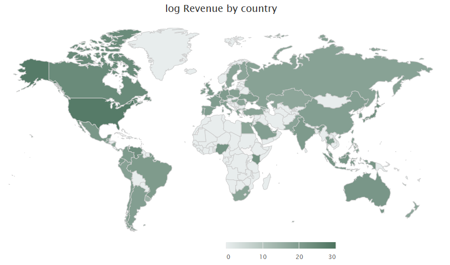
We can divide all visitors by their country information(Figure6). It shows that revenue came from all continents, with US having the highest total amount. Also, most of the hits came from US, showing the main market of Google Store is actually US rather than the whole world. Therefore the information of country might be useful in prediction revenue, but we are not sure about it.
The relation ship of log revenue with these features are visualized in Figure8. We can find weak positive relationship. This phenomenon gave evidence that these features could play important role in a statistical model.
From the analysis above, we can know that the data we have provides meaningful information about the transaction revenue, showing it is possible to predict the revenue using the data we have. Therefore we start building our statistical model.
In addition, Figure8 shows the feature importance. According to the plot, we can see that some features greatly affect
the prediction of revenue, for example: hits, pageview, visit-time and the hour time. This importance is almost the same
as the previous picture introduced in the data exploration part.
Comparing all three methods we used, we found that the tree based models(Random Forest and XGBoost) performed better than the linear model (Logistic Regression). Though Random Forest have even lower error rate than XGBoost, it misclassified too many positive samples in the test set, and therefore is not totally better than XGBoost. We will keep these two methods and compare their final performance in section5.
Each model above gave us a smaller MSE compared to predicting the average revenue, but the difference of their MSE is not significant. To compare their performance, we train these model on the same training set and ridge regression still have the lowest error rate. Therefore we will use Ridge Regression (\(\lambda\)=0.001789537) for the regression model in the whole prediction.
The final result is shown in Table6. We are already have the prior expectation that random forest will perform badly on TPR, however its bad performance(TPR=2.86%) in testing is still out of our expectation. Though random forest has a lower test error for classification, but it almost predicted all samples to be negative in test set, so we do not believe it is better than XGBoost. Therefore, XGBoost has a lowest test error in the classification period.
Table6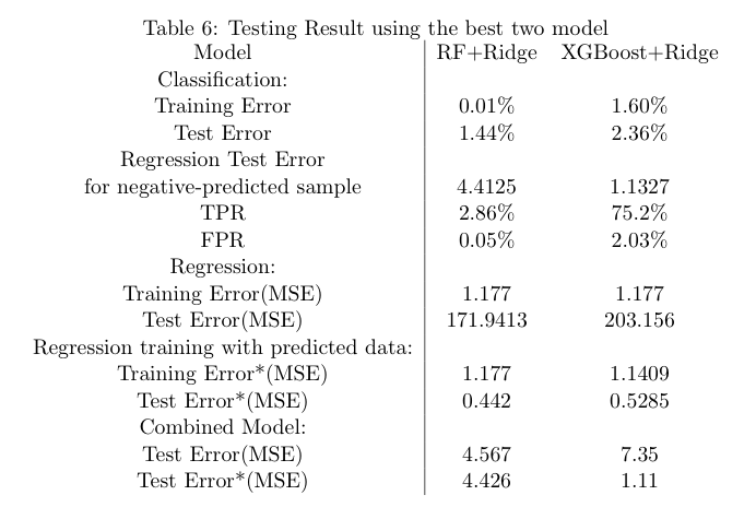 However, the higher FPR on XGBoost makes bad predictions in regression. If we use the true positive data in training set to build ridge regression model, we will have a training error of 1.177 but a much higher test error of 203.156! This high test error is caused by the false positive samples predicted in the first step. Therefore, XGBoost failed to be the better one and got a higher test error in regression. For the whole combined models on the metric of MSE, random forest plus ridge regression performed better.
Classify which device president Trump wrote his twitters
Introduction
Given the information of every twitter, the goal is to classify the device that Trump used to write each tweet with. It's been hypothesized that President Trump tweets only from his android phone and that someone else tweets from his account using an iphone.
The data file contains tweet's from President Trump's twitter from 2015 to 2016. Each row contains the text of the tweet as well as additional information such as the time that the tweet was made and the number of retweets. The column that you are predicting
is "labels" which indicates the device that the tweet was made from. In the data set the label "1" is android and "-1" is iphone. Although the tweets are publicly available through twitter,
I wan to obtain the source device for each tweet in the testing set from twitter to know which tweet is written by Trump himself.
In my point of view, there are a lot of signs that belows to Trump and other assiatant cannot mimic. For example, the sensitivity and tone from the words and also some habitual words and symbols can be
a reasonable reason to guess whether this twitter is written by Trump or someone else.
Preprocessing techniques
As eShopping becoming a more popular way to get what people need these days, online sellers found that the 80/20 rule true also on their business: only a small percentage of customers produce most of the revenue.
The dataset provides comprehensive visiting information of the online Google Merchandise Store for more than \(900,000\) recorded visits, and we are challenged to analyze it and predict revenue per visit.
In general, to predict the revenue, our idea is to divide the problem into three steps:
- Construct some classification models to divide the visits with and without revenue
- Build several regression models, training only on the data with (or might with) revenue, to predict how much revenue a single visit is probably to produce behaviors.
- Combine the classification and regression models to get the final model.
In this report we first explore the data set, drop useless information in the data and explore the correlation between the features and the label. Then for classification we use Logistic regression and two tree based methods (Random Forest and XGBoost) to predict whether the customer spent money on the website. Cross validation are used for selecting hyper parameters for each model and we compare their performance by Mean Square Error.
For regression we try linear regression (including feature selection), tree based methods (bagging and boosting) and neural network solution. We hope to get a much smaller mean square error compared to the variance of the data.
Then we use the best models from both classification (XGboost) and regression (ridge regression) to build a combined model, and improve the result by using predicted data to train the regression model. The new hybrid model has a MSE of 1.11, which shows a good performance. We formally write down the algorithm we choose to use in the fifth part.
Exploratory Data Analysis
We are interested in our target variable. For modelling log-transformed target will be used. Only 1.27% of all visits have non-zero revenue (see Figure1). The natural log of non-zero revenue seems to have a log-normal distribution with positive skewness (Figure2). User from Social and Affiliates channels did never make profit. Referral is the most profitable channel. And most of the revenues are generated by new users rather than existed users(Figure3). Though we have the information of the visit date, there seems to have no consistent relationship between date and revenue (Figure4). So we will no longer reverse the date information while training. However, time, especially the hour, will be remained since we believe it has a high correlation with the revenue.
Figure1
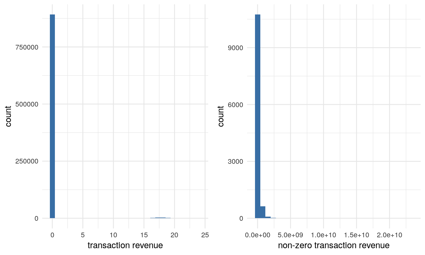
Figure2

Figure3

Figure4

We can divide all visitors by their country information(Figure6). It shows that revenue came from all continents, with US having the highest total amount. Also, most of the hits came from US, showing the main market of Google Store is actually US rather than the whole world. Therefore the information of country might be useful in prediction revenue, but we are not sure about it.
Figure5

Figure5

Figure5
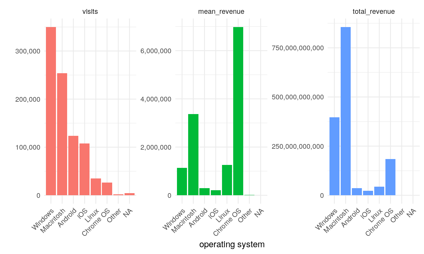
Figure6

Figure6
From the analysis above, we can know that the data we have provides meaningful information about the transaction revenue, showing it is possible to predict the revenue using the data we have. Therefore we start building our statistical model.
Figure7
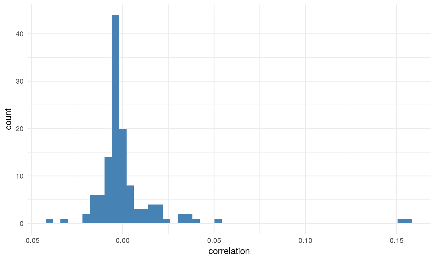
Figure8

Classification
In this part, we are working on separating the data into two disjoint part -- one part having transaction revenue and the other not.
In the classification step we replace the transaction revenue column with a binary variable showing whether revenue is made.
We use 80% of all data on training and the remaining 20% data for testing. Since the data is highly unbalanced between data
with and without revenue (almost 60:1), in all the following approaches we duplicated the data without revenue in training 60
times to make the data balance.
Actually, in the classification part, I used logistic regression, random forest, boosting and XGboost. In order to keep the report less,
I want to choose two of them (random forest and XGboost) to discuss, but I will give a comparison of all the models I create at the end of the following section.
Approach 1: Tree Based Methods
Random Forest
Compared to other methods, random forests algorithm is robust against overfitting problem. We still wanted to explore the best value of the number of sub-features(ntry). After using cross validation, we would like to choose 12 as the number sub-features. The testing error of random forest is 1.34% and training error is even as low as 0.02%! However, the FNR of the predictions on test set does not perform very well, which is higher than 1/2. In this case, we believe the error of random forest is mainly caused by high bias so that may not be the model we want to use in classification.
XGboost
Among tree based methods, bagging can help reduce variance and boosting can help reduce bias. As we have plenty of training data, variance is not as important as bias, so we prefer to use boosting. XGBoost is a popular boosting method with high training speed, and we will apply this model to our data.
Figure8
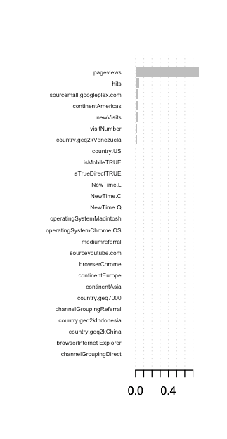
Figure9

Comparing all three methods we used, we found that the tree based models(Random Forest and XGBoost) performed better than the linear model (Logistic Regression). Though Random Forest have even lower error rate than XGBoost, it misclassified too many positive samples in the test set, and therefore is not totally better than XGBoost. We will keep these two methods and compare their final performance in section5.
Regression
After the classification, we then extract the rows whose profit is bigger than zero and fit them with regression supervised machine learning. The data with profit now only have 11843 rows. Since the profit of google store is 80/20, we know that only a small number of customers spent large amounts of money. It is therefore better to take log of those profits. We use mean square error to evaluate the performance of each model. The variance of the data with profits is 1.445991. Any model with a lower validation error is acceptable, and model with higher error rate is not better than the average prediction.
Linear Regression & Features Selection
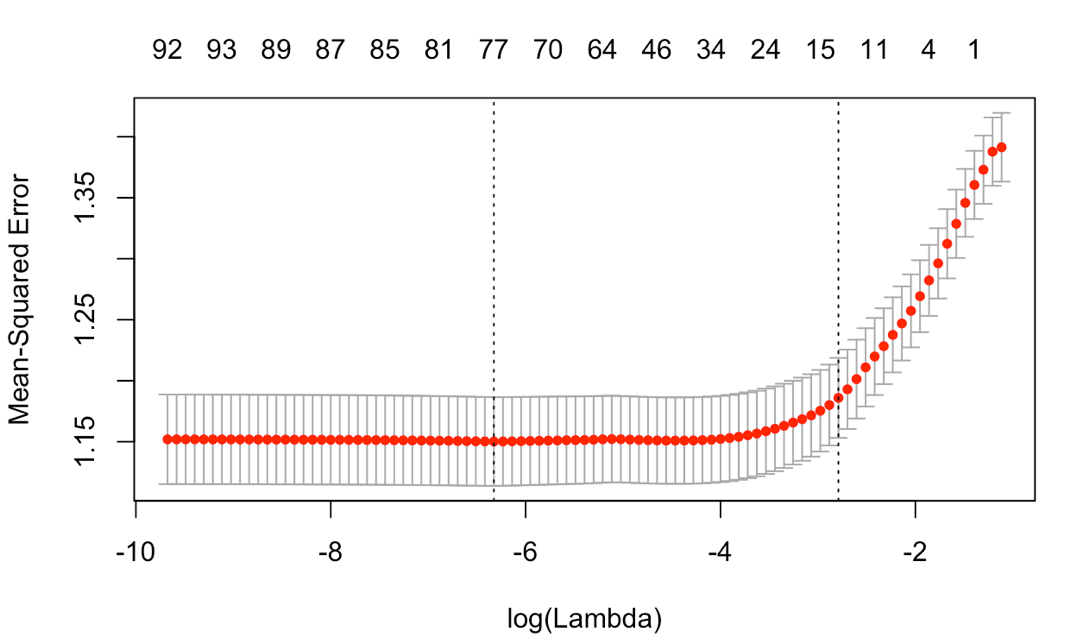
Firstly, we do a linearly regression model to have a general understanding of our data. The testing MSE is around 1.735, which is even higher than the real variance. Besides, among 53 features, only some of them are significant. Therefore, we wanted to do the features selection and find the useful and interpretable ones to rebuild a model. Considering the computation expense, we chose to use forward stepwise selection rather than best subset selection. The result shows that apart from the features like hit , pageviews , new-visit , which are also important in classification part, there still have some significant features like isMobile and browser Besides the hard selection method, we also used soft selection method: regularization. There are two types of regularization to achieve smaller flexibility: lasso and ridge. Appropriate choose of the tune parameter, \(\lambda\), can manage the bias-variance trade off very well. In order to find the optimal \(\lambda\), we do the cross validation of ridge regression and plot the CV MSE vs log(\(\lambda\)). From Figure10, we know that when \(\lambda\) equals 0.001789537 the corresponding CV error is the lowest and equals 1.147567. Besides, we also do the similar cross validation for lasso regression and the CV error achieve its lowest value (>1.15) when lambda is 0.0326147.
Figure10
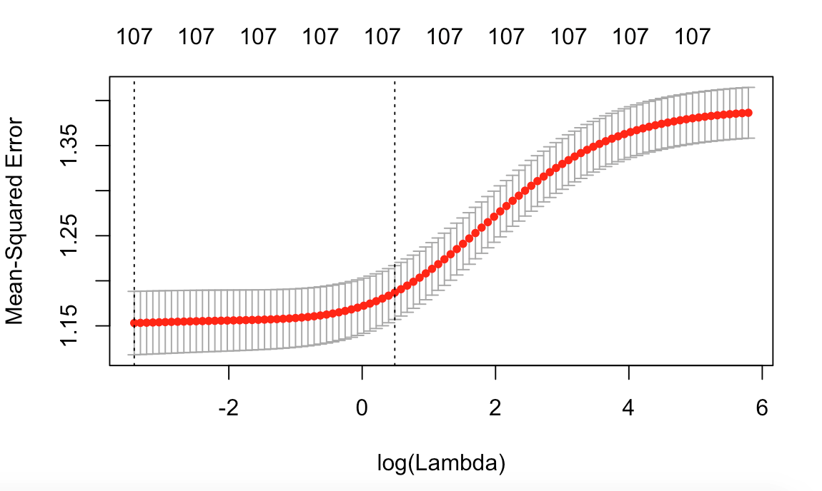
Figure10
Neural Network Structure
As been clarified in many latest papers, a deep neural network, with reasonable network structure and parameters, can fit any function arbitrarily well. That is, neural network can be trained to process prediction tasks in high accuracy with enough data. Therefore, we built a simple deep sequential neural network with 5 hidden layers and one output layer. All neighboring layers are fully connected (Structure shown as Table5. We dropped some features with huge amount of catagories and missings like region, metro, city, referralPath, keyword, networkDomain, and replace the time by time periods, and then used one-hot encoder for all catagory variables. After these steps we got 740 features in total.
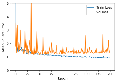
We randomly choose initial parameters, and training our neural network using Adam Optimizer several times. One of the training results after 200 epoch is shown in Figure11. The training error is generally going down, while test error has a trend of going down at first and then vibrate in a unstable level. We choose the model with lowest validation loss, which is 1.16364 as the result after 52 epochs. The corresponding training loss is 1.2208. After that, though training error continues going down, there is no positive effect on validation loss, suggesting overfitting happens. We may need different features or better net structure to enhance to result.
Table5
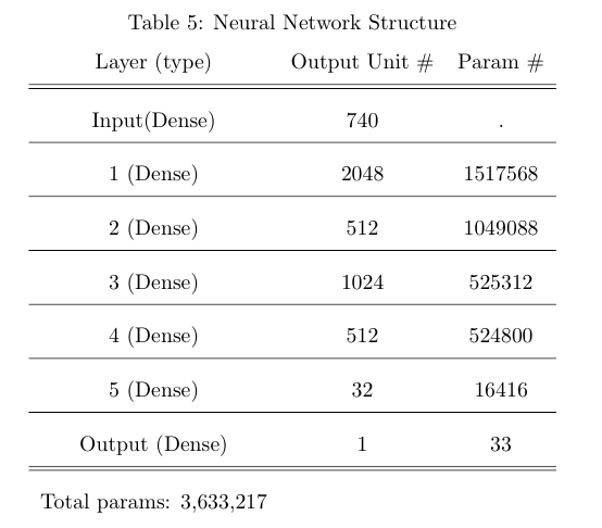
Figure11
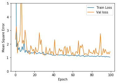
Figure11
Each model above gave us a smaller MSE compared to predicting the average revenue, but the difference of their MSE is not significant. To compare their performance, we train these model on the same training set and ridge regression still have the lowest error rate. Therefore we will use Ridge Regression (\(\lambda\)=0.001789537) for the regression model in the whole prediction.
Wrap Up Results
The final evaluation of our model will be in this form:
- Separate the data into two half (60\%+40\%) by visit time.
- Balance the non-revenue data and with-revenue data in training set by duplicating the with-revenue data 60 times.
- Train the classification model using the training set, and train the regression model use the with-revenue data in training set.
- Predict by the classification model, then predict the revenue for the positive samples by the regression model. Calculate the MSE.
The final result is shown in Table6. We are already have the prior expectation that random forest will perform badly on TPR, however its bad performance(TPR=2.86%) in testing is still out of our expectation. Though random forest has a lower test error for classification, but it almost predicted all samples to be negative in test set, so we do not believe it is better than XGBoost. Therefore, XGBoost has a lowest test error in the classification period.
Table6
However, the higher FPR on XGBoost makes bad predictions in regression. If we use the true positive data in training set to build ridge regression model, we will have a training error of 1.177 but a much higher test error of 203.156! This high test error is caused by the false positive samples predicted in the first step. Therefore, XGBoost failed to be the better one and got a higher test error in regression. For the whole combined models on the metric of MSE, random forest plus ridge regression performed better.
Conclusion and Future Study
In this study we analyzed the data of customer behavior from Google Store, and built a mixed model combining XGBoost classification and ridge regression to predict shopping behavior of every visit, which is the best model among all we have tried. Using the mixed model we can predict the log revenue with an average error of about 1, considering zero revenue visits behavior and non-zero ones are highly separative.
However, it is still hard to specifically tell how much money they will spend, since we know nothing about what they are looking for. Google now provides a new version of the data set, which contains what items visitors look through and how long they stay at each page. The richer information can help make better prediction of revenue. Next we can use these data to do future analysis, expecting to have a lower error.
On the other hand, in this study we assumed that all visits are independent and not considering relationships between visitors. For example, one might explore what he wanted to buy on his smartphone but then order by using his desktop. We can group people by their visit start time, visitor id and other information, and then consider these visits as one visit. That may help to build better predicting model.
Finally, people always wish to get prediction on what people will do rather than what they are doing. We can do further study on using existed data to predict the revenue that one customer will made in the future months. In this way Google can draft different advertising price to better serve the customers and merchants, which makes a win-win business.