Time Series / Finance
Manually using ARIMA model on predict the return on time T will involve a few steps as stated below:
Based on the factor rotation table, it can be seen that:
Mean-Reversion Portfolio Optimization with Various Return Estimation Methods
Abstract
One of the major issue of quantitative investing is that it heavily relies on the historical data. When financial market is experiencing structural changes, the historical data tend not be able to catch the changes in time. Markowitz portfolio is a very common strategy for financial investor to make trivially profitable investment strategies, and usually it assumes mean returns and covariances are given based on historical data. In this project, we compare five different methods to estimate the returns and keep using historical data for covariances to help Markowitz portfolio make a better prediction under different market circumstances. More specifically, we compare the performances of constructed portfolios when using a historical weighted estimated return, a time-series estimated return, a macroeconomic factor estimated return, and two methods of time series estimated return. The assets' returns and Sharpe Ratios of the portfolio are focused when we compare the performances of the different portfolios.
Introduction
Portfolio selection has been discussed widely across the industry for a long time, while the traditional Markowitz mean-variance optimization serves as a basic theory of portfolio selection. However, there are some controversial views against the model as well, \cite{michaud1989markowitz} points out that the accuracy of the model relies on prediction on return and variance of assets, while mean-variance optimization will "overweight those securities that have large estimated returns, negative correlations and small variances." This concern is natural since mean-variance optimization problem is largely depends on estimation of return and variance, while estimation error could be enlarged in the optimization framework. In this paper, we focus on exploring different methods of estimating return and test their performance on portfolio selection.
The paper composes with several parts as followed: The second section introduces the data collection and cleaning process. The third section introduces the basic framework of mean-variance optimization we used and four methods of estimating return, including exponential weighted model, factor model, ARIMA, and GARCH model.Also, the factor model includes a subsection explaining our factor selection using PCA method. In the fourth section we back-test the previous four models along with the equal-weighted portfolio as the benchmark on different time period. In the last part, we point out some potential directions of future works.
Data Collection and Cleaning
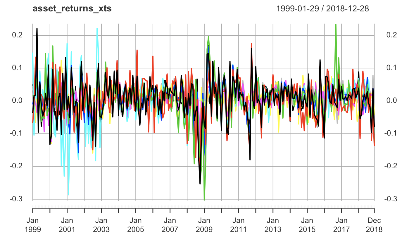
In order to construct a multi-assets portfolio, we choose nine ETFs with relatively long duration and continuous data, which includes Materials Select Sector SPDR Fund (NYSE:XLB), Energy Select Sector SPDR Fund (NYSE:XLE), Financial Select Sector SPDR (NYSE:XLF),Industrial Select Sector SPDR Fund (NYSE:XLI), Technology Select Sector SPDR Fund (NYSE:XLK), Consumer Staples Select Sector SPDR Fund (NYSE:XLP), Utilities Select Sector SPDR Fund (NYSE:XLU), Health Care Select Sector SPDR Fund (NYSE:XLV), Consumer Discretionary Select Sector SPDR Fund (NYSE:XLY). These nine ETFs reflect a wide range of assets and less sensitive to market turmoil compared to a single stock.
Beside the ETFs return data, we also need data about key fundamental marco-economics factors. Since most of the marco-economics factors are updated monthly, we consistently use monthly return in our study. We obtain monthly data from Jan 1999 to December 2018 from Yahoo Finance.
Total of 22 fundamental macro-economic factors, such as unemployment rates and consumer confidence index, were chosen initially based on monthly reports. Our team then performed a Principle Component Analysis to reduced those factors to 5 principle components.
Figure2.1
Portfolio Optimization Models
In this study, we follow the basic Markowitz mean-variance optimization framework. Using this framework, we could either minimize risk with constraints in expected return, or maximize return with some constraint in risk. For this project, we use the return maximization framework in optimization, which is calculated as following:
Actually, in the classification part, I used logistic regression, random forest, boosting and XGboost. In order to keep the report less,
I want to choose two of them (random forest and XGboost) to discuss, but I will give a comparison of all the models I create at the end of the following section.
\begin{gather*}
\text{max } \mu_0x_0 + \mu^Tx \\
\text{s.t. } xV^Tx \leq \sigma^2\\
x_0 + e^Tx + trans.cost = 1\\
x = xx+y\\
trans.cost \sum_{i=1}^n |y_i| = total.trans.cost
\end{gather*}
Risk free rate \(\mu_0\)
: Use 3-Month Treasury Bill as the indicator for risk-free rate, and do necessary transformation when we use it in monthly frequency.
Equal-weighted benchmark portfolio
: Equal weighted portfolio gives each assets in the pool the same weight, which can be used as a baseline for risk and return.
Risk constraint \(\sigma\)
: We decide sigma by multiple risk from equal weighted portfolio with an allowable risk multiplier.
Transaction cost
: Transaction costs in trading includes all kind of aspects. For ETFs, people normally consider internal costs such as management fee, external costs generated during exchange, and tax costs.
In this study, we define transaction costs as 0.005.
Initial Wealth
>: In this study, initial wealth is defined as 10000 for all models.
Restriction on the portfolio
\[abs(x - 0.1) \leq 0.05 \]
We could manually add some constraints on the optimization problem. For example, if we expect the portfolio not put too assets in one ETF, we could add a condition on CVX solver that for each assets should compose -5\% to 15\% of the portfolio.
Weighted Moving Average of Historical Return
In order to find a reliable estimation for the $\mu_T$, the most straightforward method is by adding weighted historical mean of return:
\[ \gamma: \textrm{rate of decay} \]
\[\mu_T = \frac{1}{N} ( (1-\gamma)r_{T-1} + (1-\gamma)^2 r_{T-2} + ... + (1-\gamma)^N r_{T-N})\]
This method approximates the return in time = \(T\) by using weighted moving average of previous N period of historical return, while put more emphasis on recent data than the previous one. We could expect this method gives a reliable estimation for the reason that it only gives one step ahead approximation of the return. Holding the assumption that the market will not dramatically change in a very short period, this approximation will perform nicely if the market is not experiencing huge fluctuations and the frequency historical data is relatively high.
This method is our default Mean-Variance optimization model. (We refer it later as Markowitz).
ARIMA model on return
ARIMA(p,d,q) model is a method to predict future values as linear combinations of previous data value and previous error terms. Compared to the exponential moving average method, ARIMA will choose the right amount of lag of data to include, rather than simply average over all previous weighted N data point.
To manually select the right parameters of ARIMA model, we first need to figure out if our data set is stationary. Stationary time series data has constant mean, constant variance, and finite expectation of second-order of variance. Thus, the first step will be using some techniques to transform the data set into stationary time series. Then, we could apply Autoregressive-moving-average(ARMA) model to choose the right lag and coefficient to fit the stationary time series data. Compared to simply average over a time period, ARIMA model will more precisely capture the relationship of value in time T to its previous value, thus might have better predictive power than the Weighted Moving Average method.
Figure3.1.1
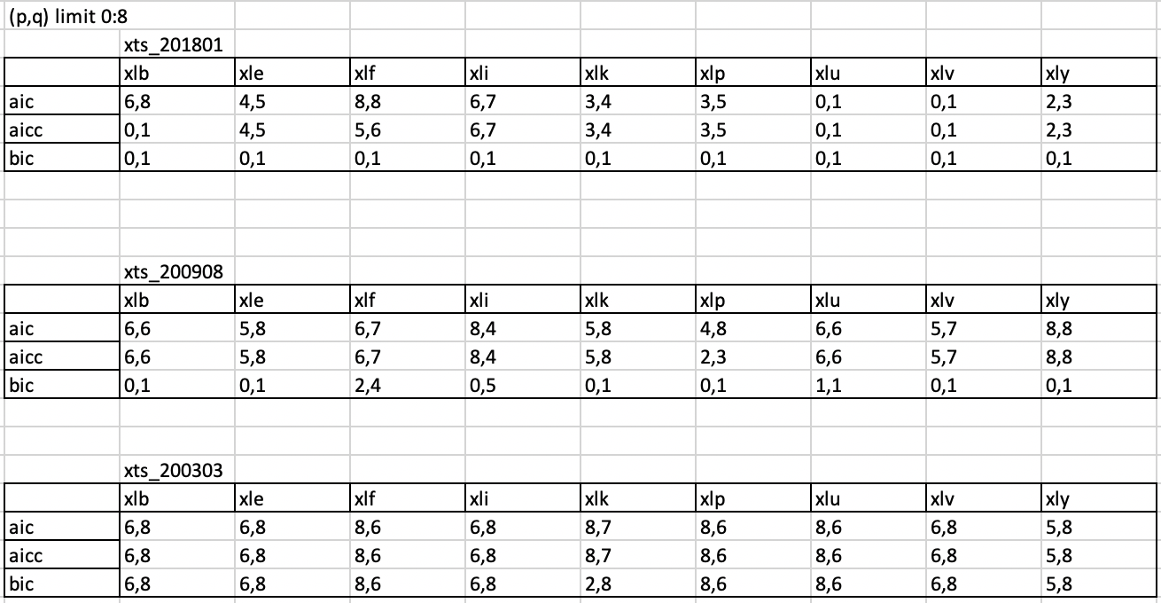
Manually using ARIMA model on predict the return on time T will involve a few steps as stated below:
- Define data as all available information before time T
- Test if the time series data is stationary using Augmented Dickey-Fuller test. If it's not, differentiates the data until it becomes stationary.
- Use AIC, AICc, or BIC as error metrics to test the differentiated time series data, and choose the order p, q of ARMA(p,q) model with lowest error metrics. (Note: AIC, AICc, and BIC might suggest different order p,q. In this study, we choose AIC when we have conflict.
- Plot ACF, PCAF graphs or use Ljung-box test on residuals to confirm the current model already capture all the auto-correlations. Otherwise, choose a higher order of p,q.
GARCH model on return
Although ARIMA model could handle non-stationary in mean, it doesn't work well with non-stationary variance which is very common in financing data. In GARCH model, it incorporate variances as a changing variable in predictions. It represents the reality in ETF returns that during market turmoil the variance can be extremely high,
while in other time the variance may stay relatively stable. The equation of GARCH(m,r) could be written as:
\[ x_t = \sigma_t e_t \]
\[ \sigma_t^2 = \alpha_0 + \alpha_1x_t^2 + .... + \alpha_mx_{t-m}^2 + \beta_1\sigma{t-1}^2 + ... + \beta_r\sigma{t-r}^2\]
In our study, we choose GARCH(1,1) as our prediction tools for the return.
Macroeconomic factor models
Since there are in total 9 ETF assets, the factors we choose could not exceed that number to avoid over-fitting. In order to take all 22 factors into consideration, we perform Principal Component Analysis to reduce the dimension of our factors.
Principle Component Analysis
The monthly returns of all the factors have been calculated first. We choose 5 principal components, and from principle component 1 to principle component 5,
we find they could explain 0.592, 0.235, 0.069, 0.059 and 0.021 of total variance, respectively. These five principle components can explain 97.6% total variance of the return data.
According to the non-unique line of the factor load matrix, the factor rotation can be performed so that each variable has a large load on the unique factor for common factor analysis.
From the partial load matrix after rotation below, the absolute value of maximum load factors of initial features for each principle components has been used to determine which principle
component the initial factors could be classified as. The complete version of transformed loading matrix can be found in appendix.
Figure3.4.1.1
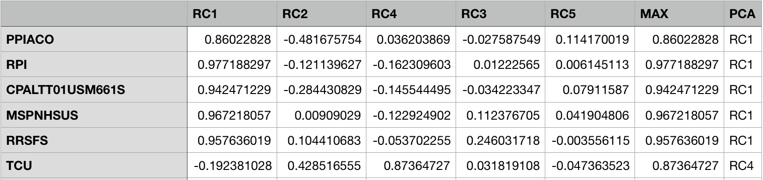
Based on the factor rotation table, it can be seen that:
- Factor F1 has large loadings on Producer Price Index for All Commodities, Real Personal Income, Consumer Price Index, Median Sale Price for New Houses Sold in US, etc. The above macroeconomic indicators are related to the market's sales and production levels; therefore, we name RC1 as sales and production.
- Factor RC2 has large loadings on Consumer Comfidence Index, New Private Housing, Consumer Sentiment, and Number of initial insurance claims. These indicators are related to the market's consumer confidence, which make RC2 can be named as the consumer confidence indicator.
- Factors RC3 includes goods and service trade balance. Therefore, it will still be named as goods and service trade balance.
- Factor RC4 has large loadings on total capacity utilization. We then name RC4 as capacity utility.
- Only unemployment ratio may be included in factors RC5. RC5 is named as unemployment ratio.
Applying PCA to factor model
In factor model, there are several parameter to decided. We decide to test the rebalance start date from 90, 100 and 120 after the first day of the data set and try to set number of sample to 20 and 50 in computing return averages and covariances matrix. We choose the horizon to be 1 (one month) since our data is in monthly frequency. The number of the total macro economics factors is 22, thus we perform PCA linear combination of different macro factors to condense to 5 principal component factors.
The basic equation for the factor model is:
\begin{gather*}
r_i = \alpha_i + \sum_{j=1}^{m}\beta_{ij}f_i+\epsilon_i\\
\mu = \alpha + BE(f)\\
V = BFB^T + \Delta
\end{gather*}
Since marco-economics factor returns after PCA manipulation\(f\) and actual returns \(r\) are observable, we need to calculate out \(alpha\), \(epsilon\), \(beta\) first, and then calculate delta, mean and covariance correspondingly.
In this project, we capture the relationship between assets returns and macro economics factors' returns by using linear regression, then store the information in \(alpha\), \(epsilon\), and \(beta\). Using the stored information, we are able to calculate mean and variance. The calculation is done iterative during each rebalance, and each time we move the windows of assets returns and macro economics factors' returns by frequency we specify (1 month).
Marco-economics factor model is also compared to original Mean-Variance optimization and equal-weighted benchmark. All these models are under the same parameter conditions so we could compare the performance across models.
Testing Results
We have already built three mean prediction models: ARIMA, GARCH and PCA marco-economics factor model. We want to compare the performance of these three models and two benchmark models described before (Markowitz model and equal weighted benchmark model). The performance of these models is different according to different parameters (start time, sample time window and number of rebalance time).
Special period analysis
Considering 2008 financial crisis, it is a special period that need to pay attention to. From the figure 4.1.1 below, we choose the start day from January 2006
and look at the performance of five different models. There is a dramatic drop in the 32th month from January 2006, which is 2008 financial crisis period.
In general, the wealth of all models is decreasing. However, among these models, the amount of decreasing of Markowitz (the yellow line) model is the smallest,
followed by ARIMA, factor model, benchmark. The worst performance during this period is GARCH model. Moreover, the wealth difference between GARCH and other models
is very large. The main reason could be GARCH model is quite "aggressive" since the model itself will adjust the lag value no matter the number of sample
(time window) changes. The output shows that GARCH model performs poorly in fluctuated period. However, after the crisis, the GARCH model recovers back and
over-performs benchmark and factor model around peirod 90.
In this time period, the Markowitz model has a consistently good performance in 2008 and other months. The wealth from Markowitz model stays high in 2008 crisis and it remains as the best performer after that, followed by ARIMA, GARCH and benchmark models.
Regarding the factor model, although it performs better than the benchmark model in 2008, it gradually becomes the worse among the five models. This reason might be the factor model contains some leading macro economics factors that could forecast some future unknown issues. It is a conservative method of predicting returns and thus performing better during recession but extremely bad on expansion. The model is also too pessimistic to stack on some high risk but high return assets.
In conclusion, the Markowitz model is consistently the best in most of the time, while the GARCH model perform worst during market turbulence. The GARCH model, however, can quickly adjust during economic expansion. The factor model is performing well during 2008 crisis, but it could have the worse performance compare to other models under a stable market condition.
Figure4.1.1

Different investment start time
To an investor, choosing different starting time to invest could result in quite different wealth in the future while using same model to predict. From figure 4.2.1, the investment is starting at 2009 while in 4.1.1 the investment is starting at 2006. The period in figure 4.1.1 includes year 2008. The results from two different investment starting time are quite different.
If we start investment from 2009, the overall financial environment is warming up, making GARCH model becomes the best model among all others. The wealth difference between GARCH model and other models is growing larger and larger for every consecutive year. Markowitz and ARIMA model follow as the second and the third, while the worst model is still PCA factor model.
As mentioned before, GARCH model adjusts quickly to the good financial environment, so in the long run, GARCH will present good predictions in a stable financial market. Also because of the "aggressive" property of GARCH, the return of using this model is very attracting.
However, in this starting point of investment, Markowitz model has mediocre performance compared to the previous case. It could be explained that without the advantages of wealth accumulated during 2008 crisis, Markowitz has no major advantages over benchmark model and ARIMA model.
The Figure 4.3.2 below summarizes 6 different tests and its results of final wealth. Observing the table we could find that the investment started from 2006 is the lowest, then 2007, and the highest wealth is from 2009. It's because 2008 economic recession decreases the investment wealth a lot and later wealth need to cover the loss.
Figure4.2.1

Different time window (number of samples chosen to calculate mean and covariance)
We set different number of samples to calculate the mean and variance in this study. In factor model, number of samples could affect the result of the coefficient,
constant and residuals of linear regression. For Markotiz model, the number of samples could affect the prediction of weighted average of mean and variance.
According to figure 4.3.1 and figure 4.1.1, the model rank based on the the wealth over 2006 to 2008 is not affected by the difference between sample size.
In other words, Markowitz model is the best model, followed by ARIMA, GARCH, benchmark and PCA factor model. The only difference is the small total wealth difference:
From figure 4.3.2, not only the total final investment wealth of sample 50 is always smaller than that of sample 20, but also the annualized rate of return.
The main reason could be that size 50 (more than 4 years) is too long to be used to predict the future return. Using size 20 could capture more recent market change
and information, which could predict the future risk asset returns better compare to use size 50.
To sum up, use different length of time window to calculate mean and covariance would not affect the rank of model performance under the three scenario we test, but could result in different prediction on return and then influence the final investment wealth.
However, in this starting point of investment, Markowitz model has mediocre performance compared to the previous case. It could be explained that without the advantages of wealth accumulated during 2008 crisis, Markowitz has no major advantages over benchmark model and ARIMA model.
The Figure 4.2.1 below summarizes 6 different tests and its results of final wealth. Observing the table we could find that the investment started from 2006 is the lowest, then 2007, and the highest wealth is from 2009. It's because 2008 economic recession decreases the investment wealth a lot and later wealth need to cover the loss.
Figure4.3.1
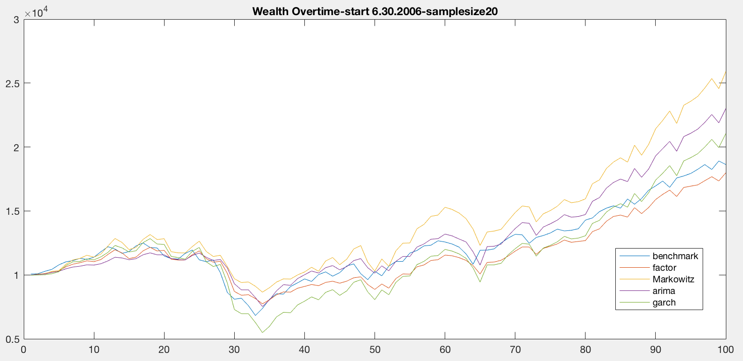
Figure4.3.2

Conclusion
- Regarding GARCH model, we currently use GARCH(1,1) to all the data set. One problem with this approach is that it might still encounter non-stationarity in mean. Thus, one potential improvement could be applying augmented Dickey Fuller test and differentiating the data to make sure it's stationary in mean. Another potential improvement could be choose the m, r order for GARCH more precisely for each time period and each assets.
- Choosing factors is a major part of the factor model. One disadvantage of PCA is the lack of interpretability. Thus, we could compare PCA with other traditional methods such as using regressions with considerations of correlation.
- It's known that a major advantage of marco-economics factor model is requiring less data for co-variance matrix during calculation. In order to get a more reliable estimation of mean, we could use Black-Litterman model further to improve the factor model.
- Most of the marco-economics factors are in monthly frequency. In order to be consistent during our analysis, we apply monthly data for all five models. It could be better if we use data with higher frequency to check the performance of ARIMA and GARCH model in future work.
Future Work
Applying these five models to estimate return, we find that there doesn't exist an absolute best prediction across all time period and different setting in parameters. If the market does not experience huge turbulence in time, GARCH model will give the best performance on portfolio selection. The performance of Markowitz is good overall under the monthly frequency of data, with better results in financial market turmoil. PCA factor models, however, does not perform well in the long run. In general, PCA takes account all the factor into consideration instead of choosing important factor which are related to the asset returns. Although PCA performs well in explaining total variance and avoid correlation, it doesn't make PCA a good factor selection tool. ARIMA model also fails to outperform Markowitz model. It might because exponential averaging technique performs well in one-step-ahead scenario. ARIMA is more conservative than GARCH model, but has no substantially more predictive power than exponential averaging estimate of return.